10.2. Application MonitoringWe can imagine our statistics in a stack similar to the OSI seven-layer network model. At the top of our stat stack are the application-level statistics, as shown by our dashboard. These give an overview of usage at the application level, abstracted to represent operations at a level that would be understood by a user of the application. This might include how many discussion topics were created, how many users have registered accounts, and so on. The second layer from the top of our stack is comprised of web statistics, the stats one logical layer beneath the general application. This includes user behavior in the form of path tracking as well as request volume. So what comes lower? Getting into the transport layers in the middle of our stack, we have internal application service statistics. This would typically be comprised of components such as Apache, MySQL, memcached, and Squid. This layer could include MySQL query statistics, Apache memory statistics, or memcached cache hit rates. Below the transport layers comes the network layer, which is comprised of OS-level statistics. This could include CPU usage, memory utilization, interrupts, swap pages, and process counts. At the very bottom of our stack come low-level hardware statistics. How fast is the disk spinning? How hot is the processor? What's the status of the RAID array? So how can we get statistics for these bottom layers? For managers and executives, the top layers are usually the most important, but as engineers, we should care more about the layers below. To know if a service is functioning and how well it's performing, we really need statistics about that service in particular, rather than global usage statistics. Long-term statistical data about the components in our system allows us to more easily spot emerging trends in usage as well as performance information. If we're tracking the idle processor time on a machine and it's gradually trending toward zero, then we can spot the trend and plan for capacity: at the growth rate we're seeing, we'll need more processor power in X days. This kind of statistic can then be built into your dashboard and used for capacity planning. With detailed usage data, you can spot and remedy bottlenecks before they have an impact on your operations. So we know we need to gather these statistics to help get a better understanding of what's going on in the guts of our application. But how should we go about this? We're going to need some more tools. 10.2.1. Bandwidth MonitoringThe Simple Network Management Protocol (SNMP) allows us to query network devices for runtime information and statistics. You can use SNMP to poke your switch and ask it how much data it's pushed through a specific port. Switches typically return a single numberthe number of bytes they pushed through since they were last restarted. By recording this number at regular intervals, we can calculate the difference and plot how much data moved through the switch port during each sampling period. Not all switches support SNMP or track the data you'd need, but nearly all routers do. Since there's a router port somewhere between your servers and the Internet, you can query it (or your host can if it's shared among multiple hostees) to find out your total incoming and outgoing data rate. The Multi-Router Traffic Grapher (MRTG) allows you to easily create bandwidth usage graphs from SNMP data, as shown in Figure 10-5. Figure 10-5. A bandwidth usage chart created from data collected via SNMP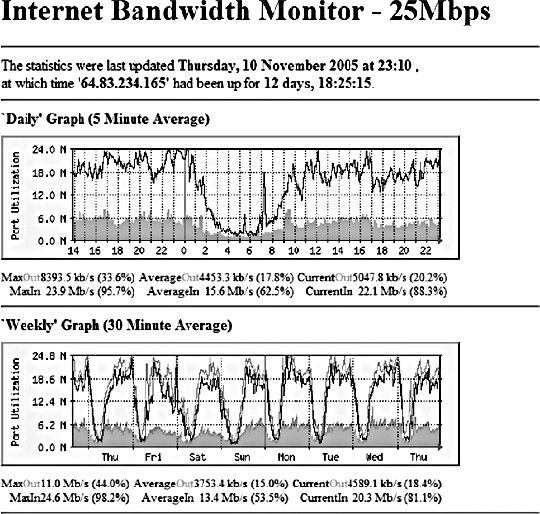 To install MRTG, simply download a copy (http://mrtg.hdl.com/), compile it, and point it at your router. You'll need to know the community name of your router (try "public" first) and the IP address of its local interface. After generating a configuration file, you need to set MRTG to be run every five minutes, or however often you want updates. Each time it runs, MRTG will go and fetch the traffic counts, store them in its database, and update the graphs. MRTG uses something called a round robin database that always stores a fixed amount of data. As data gets older, it's averaged over a longer time period. Data from the last day contains a sample for every 5 minutes, while data for the last week contains an averaged sample for every 35 minutes. Because of this, we can continue logging data indefinitely without ever having to worry about running out of disk space. The downside, of course, is that we lose high-resolution data from the past. For bandwidth monitoring, this isn't usually such a bad thing, as current events and long-term trends are what we care about. The other downside is that, by default, we'll lose data over a year old. For long-running applications, this can become a problem. To get around this limitation, we can use RRDTool, a successor to MRTG that allows many more options. We'll look at this in a moment. 10.2.2. Long-Term System StatisticsWhile bandwidth usage is very exciting, after about 30 seconds of looking at MRTG graphs, you're going to become starved for information. MRTG follows the Unix principle of doing one thing and doing it well, but we want to monitor a bunch of other things. Ideally, we want what's known as data porn . In practical terms, data porn loosely describes having more data available for analysis than you need. In practice this means collecting information from every low-layer element of your entire system, graphing it, and keeping historical data. One of the problems with doing this is that it takes a lot of space. If we capture a 32-bit statistic once every minute for a day, then we need 11.2 KB to store it (assuming we need to store timestamps, too). A year's worth of data will take 4 MB. But remember, this is for one statistic for one machine. If we store 50 statistics, then we'll need 200 MB. If we store this data for each of 50 machines, then we'll need 9.7 GB per year. While this isn't a huge amount, it continues to grow year on year and as you add more hosts. The larger the data gets, the harder it gets to interpret as loading it all into memory becomes impossible. MRTG's solution to this is fairly elegantkeep data at a sliding window of resolution. The database behind MRTG stays exactly the same size at all times and is small enough to keep in memory and work with in real time. The database layer behind MRTG was abstracted out into a product called RRDTool (short for round robin database tool), which we can use to store all of our monitoring data. You can download a copy and see a large gallery of examples at http://people.ee.ethz.ch/~oetiker/webtools/rrdtool/. A typical RRD database that stores around 1.5 years of data at a suitable resolution for outputting hourly, daily, weekly, monthly, and yearly graphs takes around 12 KB of storage. With our example50 statistics on 50 nodeswe'll need a total of 28 MB of space. This is much less than our linear growth dataset size and gives us plenty of room for expansion. This gets us out of the situation of ever deciding not to monitor a statistic due to storage space concerns. We can use RRDTool for our data storage, but we still need to deal with collecting and aggregating the data. If we have multiple machines in our system, how do we get all of the data together in one place? How do we collect the data for each statistic on each node? How do we present it in a useful way? Ganglia (http://ganglia.sourceforge.net/) takes a stab at answering all of these questions. Ganglia is comprised of several components: gmond, gmetad, and gmetric (pronounced gee-mon-dee and so forth), which perform the roles of sending data, aggregating data, and collecting data, respectively. gmond, the Ganglia-monitoring daemon, runs on each host we want to monitor. It collects core statistics like processor, memory, and network usage and deals with sending them to the spokesperson for the server cluster. The spokesperson for a cluster collects all of the data for the machine in a cluster (such as web servers or database servers) and then sends them on to the central logging host. gmetad is used for aggregating together cluster data at intermediate nodes. gmetric allows you to inject extra metric data into the Ganglia multicast channel, sending your statistics to the central repository. One of the concerns for statistical data collection, especially across a system with many nodes, is that constantly requesting and responding with metric data will cause excessive network traffic. With this in mind, Ganglia is built to use IP multicast for all communications. Unlike logging, we don't really care if we drop the odd statistic on the floor as long as enough data reaches the logging node to be able to graph the statistic with reasonable accuracy. Because we're using multicast, we can avoid the number of needed connections growing exponentially and allow multiple machines to collect the multicast data without adding any extra network overhead. At the point of data collection, Ganglia, shown in Figure 10-6 and Figure 10-7, uses RRDTool to create a database file for each statistic for each host. By default, it also automatically aggregates statistics for each cluster of machines you define, letting you get an overall view of each statistic within the clusterfor instance, the cumulative network I/O for your web servers or memory usage for your database cluster. For managing huge setups, Ganglia can also collect clusters together into grids, allowing you to organize and aggregate at a higher level again. Figure 10-6. A Ganglia report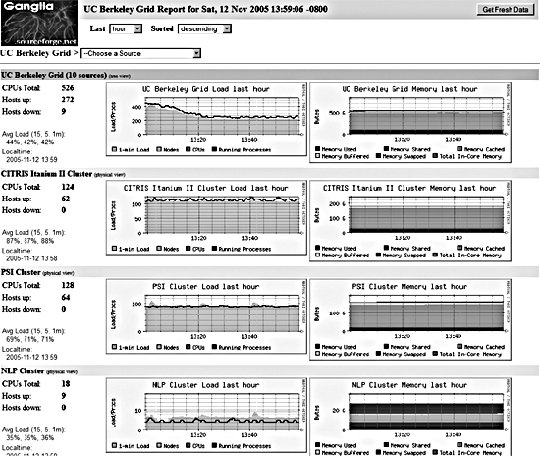 Figure 10-7. A different Ganglia report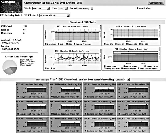 One of the really useful abilities of the Ganglia system is how easy it is to extend the monitoring with custom metrics. We can write a program or script that runs periodically via cron to check on our statistic and then feed it into the Ganglia aggregation and recording framework by using the gmetric program. Our custom scripts can collect the data using whatever means necessary and then inject a single value (for each sampling run) along with the metric they're collecting for, its format, and units: /usr/bin/gmetric -tuint32 -nmemcachced_hitratio -v92 -u% This example feeds data into Ganglia for a statistic called memcached_hitratio. If Ganglia hasn't seen this statistic before, it will create a new RRDTool database for storing it, using the data type specified by the -t flag (unsigned 32-bit integer in this example). The value 92 is then stored for this sampling period. Once two sampling periods have been completed, we can see a graph of the memcached_hitratio statistic on the Ganglia status page for that node. The final -u flag lets us tell Ganglia what units the statistic is being gathered in, which then displays on the output graphs, as shown in Figure 10-8. Figure 10-8. Output graph with units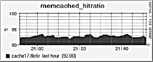 Depending on the components in your system, there are lots of useful custom statistics that you'll want to consider collecting and graphing. We'll look at each of the common major components of a web-based application and suggest some statistics you might want to collect and how you would go about finding them. 10.2.2.1. MySQL statisticsFor MySQL servers, there are a few really useful statistics to track. By using the SHOW STATUS, we can extract a bunch of useful information to feed into Ganglia. The Com_* statistics give us a count of the number of each query type executed since MySQL was started. Each time we run our stats collection, we can note the value for Com_select and friends. On each run, we can then compare the new value against the old value and figure out how many queries have been run since our last sample. Graphing the Select, Insert, Update, and Delete count will give you a good idea of what kind of traffic your server is handling at any point in time. We can perform basic service-level checks too, which can be useful for longer term statistics gathering. If we can connect to MySQL, then we can set the value for mysql_up to 1, or set it to 0. We then get a long-term graph of MySQL uptime and downtime on each database node. Although Ganglia tracks general machine uptime, we may sometimes want to track specific services (such as MySQL) since the service can be down while the rest of the node is up. MySQL has a hard connection thread limit, which when reached will block other client processes from connecting. In addition there is also a thread cache setting that determines how many threads MySQL keeps around ready for incoming connections to avoid thread creation overhead. We can graph the number of active connections by using the SHOW PROCESSLIST command to get a list of all the currently open threads. We can then look at this number against the maximum thread limit and the cached threads setting. If the number of open connections is consistently higher than the number of cached threads, then we would benefit from increasing the cached threads. Conversely, if the number is consistently lower, then we can reduce the number of cached threads to save memory. If the number of open connections is nearing the connection limit, then we know we'll either need to bump up the connection limit or that something is going wrong with our system in general. If we're using replication in our system, then there are a few additional statistics we can gather. At any time, each thread should have two threads open to the master. The I/O thread relays the master's binary log to the local disk, while the SQL thread executes statements in the relay log sequentially. Each of these threads can be running or not, and we can get their status using the SHOW SLAVE STATUS command. More important for graphing is the replication lag between master and slave (if any). We can measure this in a couple of ways, both of which have their advantages and disadvantages. We can look at the relay log write cursor and execution cursor using the SHOW SLAVE STATUS command and compare the two. When they both point to the same logfile, we can look at the difference between the two cursors and get a lag value in binlog bytes. When they point to different logs, we have to perform some extra calculations and have to know the size of the master's binlogs. While there's no way to extract this information at runtime from the slave (without connecting to the master, which is probably overkill for monitoring, especially if we have many slaves), we will typically have a single standard binary log size across all of our database servers, so we can put a static value into our calculations. For example, assume we use 1 GB (1,073,741,824 bytes) binary logs and the output from SHOW SLAVE STATUS looks like this:
mysql> SHOW SLAVE STATUS \G
*************************** 1. row ***************************
          Master_Host: db1
          Master_User: repl
          Master_Port: 3306
        Connect_retry: 60
      Master_Log_File: db1-bin.439
  Read_Master_Log_Pos: 374103193
       Relay_Log_File: dbslave-relay.125
        Relay_Log_Pos: 854427197
Relay_Master_Log_File: db1-bin.437
     Slave_IO_Running: Yes
    Slave_SQL_Running: Yes
      Replicate_do_db:
  Replicate_ignore_db:
           Last_errno: 0
           Last_error:
         Skip_counter: 0
  Exec_master_log_pos: 587702364
      Relay_log_space: 854431912
1 row in set (0.00 sec)
The Master_Log_File value tells us which file the I/O thread is currently relaying, while the Read_Master_Log_Pos value tells us what position in the file we've relayed up to. The Relay_Master_Log_File value tells us which file we're currently executing SQL from, with the Exec_master_log_pos value telling us how far through the file we've executed. Because the values for Master_Log_File and Relay_Master_Log_File differ, we know that we're relaying a newer file than we're executing. To find the lag gap, we need to find the distance to the end of the file we're currently executing, the full size of any intermediate relays logs, and the portion of the latest relay log we've relayed. The pseudocode for calculating the slave lag is then as follows:
if (Master_Log_File == Relay_Master_Log_File){
        slave_lag = Read_Master_Log_Pos - Exec_master_log_pos
}else{
        io_log_number  = extract_number( Master_Log_File )
        sql_log_number = extract_number( Relay_Master_Log_File )

        part_1 = size_of_log - Exec_master_log_pos
        part_2 = ((io_log_number - sql_log_number) - 1) * size_of_log
        part_3 = Read_Master_Log_Pos
        slave_lag = part_1 + part_2 + part_3;
}
Our I/O and SQL thread logs aren't the same, so we need to use the second code block to figure out our lag. For the first portion, we get 486,039,460 bytes. For the second portion, we have a single log between the I/O (439) and SQL (437) logs, so we get 1,073,741,824 bytes. Adding the third part of 374,103,193, we have a total lag of 1,933,884,477 bytes, which is roughly 1.8 GB. Ouch. Until you get a good idea for how much of a lag 1.8 GB is, there's a second useful method for getting an idea of lag. When we run the SHOW PROCESSLIST command on a slave, we see the SQL and IO threads along with any regular client threads:
mysql> SHOW PROCESSLIST;
+-----+-------------+--------+------+---------+---------+-------------+-------------+

| Id  | User        |  Host  | db   | Command | Time    | State       | Info
  |
+-----+-------------+--------+------+---------+---------+-------------+-------------+

| 1   | system user |        | NULL | Connect | 2679505 | Waiting     | NULL
                                                          for master
  |
| 2   | system user |        | Main | Connect | 176     | init        | SELECT * FROM
                                                                        Frobs
|
| 568 | www-r  | www78:8739  | Main | Sleep   | 1       |             | NULL
  |
| 634 | root   | admin1:9959 | NULL | Query   | 0       | NULL        | SHOW
                                                                        PROCESSLIST
  |
+-----+-------------+--------+------+---------+---------+-------------+-------------+
The first thread is the I/O thread, while the second is the SQL thread. They don't always appear first in the process list if they were started after MySQL or if they've been restarted since, but you can scan down the thread list to find threads with a user of system user. We can then look at the db field to find out whether we're looking at an I/O or SQL thread. The I/O thread doesn't connect to a specific database, so we can identify it by a NULL value in this column. The SQL thread can also have a NULL value when it's finished replicating, but we can identify it because in this case it'll have the special status "Has read all relay log; waiting for the I/O slave thread to update it." If we find a thread owned by system user with a database specified, then we know that it's the SQL thread and that it's not caught up to the I/O thread. In this case, the Time column has a special meaning. Usually it contains the time the thread has been executing the current statement. For the I/O thread, it contains how long the I/O thread has been running in seconds (just over 31 days in our example). For the SQL thread, it contains the time since the currently executing statement was written to the master's binary log. We can use this value to measure slave lag since it tells us how long ago the currently relaying statement was issued to the master. In this way, we can say our example server has 176 seconds of replication lag. This doesn't mean that it'll take 176 seconds to catch up, just that it's 176 seconds behind the master at this moment in time. A slave with more write capacity will catch up faster, while a slave with less write capacity than the traffic currently running on the master will continue to fall behind and the number will increase. 10.2.2.2. Apache statisticsmod_status allows you to easily extract runtime statistics from Apache. It's often installed by default and serves statistics at the /server-status/ URL. Access to this URL is by default restricted to localhost in the Apache configuration using the following configuration block:
<Location /server-status>
        SetHandler server-status
        Order deny, allow
        Deny from all
        Allow from localhost
        Allow from 127.0.0.1
</Location>
If we lift these restrictions and look at the page in a browser, we see some useful statistics and a table of all current threads, their status, and details of the last request they served. For getting information out in an easily parsable format, mod_status has an "automatic" mode, which we can activate with the auth query string. Using the wget utility on the command line, we can easily summon the server status: [calh@www12 ~] $ wget -q -O - http://localhost/server-status/?auto Total Accesses: 27758509 Total kBytes: 33038842 CPULoad: .154843 Uptime: 1055694 ReqPerSec: 26.2941 BytesPerSec: 32047 BytesPerReq: 1218.79 BusyWorkers: 59 IdleWorkers: 28 Scoreboard: _K__CK_K__CKWKK_._KW_K_W._KW.K_WCKWK_.KKK.KK_KKK_KK_ _CKKK_KK KK__KC_ _.K_CK_KK_K_...KCKW.._KKK_KKKK...........G........... ............................................................ ............................................................ ............................................................ ............................................................ ............................................................ ............................................................ ............................................................ ............................................................ ............................................................ ............................................................ ............................................................ ............................................................ ............................................................ ............................................................ ............................................................ .... The most interesting statistics for us here are the total accesses and kilobytes transferred. By sampling this data once a minute and recording the values, we can log the delta into Ganglia and see the exact number of requests served every minute along with the bandwidth used. Graphing this value over time, we can see how much traffic is hitting each server. We can also track the busy and idle worker processes to see how many requests we're servicing at any one time and how much process overhead we have at any time, as shown in Figure 10-9. If this value often hits zero, then we need to increase our MinSpareServers settings, while if it's consistently high, then we can decrease it to save some memory. Figure 10-9. Monitoring process overhead in Ganglia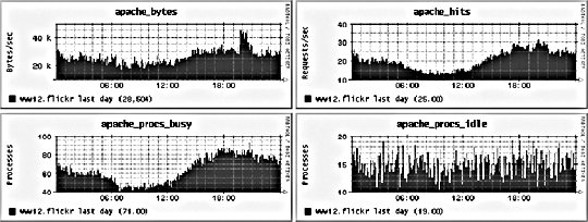 These graphs tell us that we're serving an average of about 20 requests per second throughout the day (1.7 million total), with a low of 15 and a high of 30. Our idle processes never really dips below 10 (as it shouldn'tthat's our MinSpareServers setting), but we'd want to check a more fine-grained period (such as the last hour) to see if we're ever reaching zero. If not, we could probably safely reduce the number of spare processes to gain a little extra performance. 10.2.2.3. memcached statisticsmemcached has a command built into its protocol for retrieving statistics. Because the protocol is so simple, we can make an API call and fetch these statistics without having to load a client library. In fact, we can run the needed commands using a combination of the Unix utilities echo and netcat: [calh@cache7 ~] $ echo -ne "stats\r\n" | nc -i1 localhost 11211 STAT pid 16087 STAT uptime 254160 STAT time 1131841257 STAT version 1.1.12 STAT rusage_user 1636.643192 STAT rusage_system 6993.000902 STAT curr_items 434397 STAT total_items 4127175 STAT bytes 1318173321 STAT curr_connections 2 STAT total_connections 71072406 STAT connection_structures 11 STAT cmd_get 58419832 STAT cmd_set 4127175 STAT get_hits 53793350 STAT get_misses 4626482 STAT bytes_read 16198140932 STAT bytes_written 259621692783 STAT limit_maxbytes 2039480320 END This command connects to the local machine on port 11211 (the default for memcached) and sends the string stats\r\n. memcached then returns a sequence of statistic lines of the format STAT {name} {value}\r\n, terminated by END\r\n. We can then parse out each statistic we care about and graph it. By storing some values between each sample run, we can track the progress of counters such as total_connections and get_hits. By combining statistics such as bytes and limit_maxbytes, we can graph how much of the system's total potential cache is in use. By looking at the difference between curr_items and total_items over time, we can get an idea of how much the cache is churning. In the above example, the cache currently stores about 10 percent of the objects it's ever stored. Since we know from uptime that the cache has been alive for three days, we can see we have a fairly low churn. 10.2.2.4. Squid statisticsIf you're the kind of person who finds data porn awesome, then not many system components come close to Squid's greatness. Using the Squid client program, we can extract a lot of great runtime information from our HTTP caches. The info page contains an all time information summary for the Squid instance:
[calh@photocache3 ~] $ /usr/sbin/squidclient -p 80 cache_object://localhost/info
HTTP/1.0 200 OK
Server: squid/2.5.STABLE10
Mime-Version: 1.0
Date: Sun, 13 Nov 2005 00:37:08 GMT
Content-Type: text/plain
Expires: Sun, 13 Nov 2005 00:37:08 GMT
Last-Modified: Sun, 13 Nov 2005 00:37:08 GMT
X-Cache: MISS from photocache3.flickr
Proxy-Connection: close
Squid Object Cache: Version 2.5.STABLE10
Start Time:     Tue, 27 Sep 2005 20:41:37 GMT
Current Time:   Sun, 13 Nov 2005 00:37:08 GMT
Connection information for squid:
        Number of clients accessing cache:      0
        Number of HTTP requests received:       882890210
        Number of ICP messages received:        0
        Number of ICP messages sent:    0
        Number of queued ICP replies:   0
        Request failure ratio:   0.00
        Average HTTP requests per minute since start:   13281.4
        Average ICP messages per minute since start:    0.0
        Select loop called: 1932718142 times, 2.064 ms avg
Cache information for squid:
        Request Hit Ratios:     5min: 76.2%, 60min: 75.9%
        Byte Hit Ratios:        5min: 67.4%, 60min: 65.8%
        Request Memory Hit Ratios:      5min: 24.1%, 60min: 24.0%
        Request Disk Hit Ratios:        5min: 46.5%, 60min: 46.7%
        Storage Swap size:      26112516 KB
        Storage Mem size:       2097440 KB
        Mean Object Size:       22.95 KB
        Requests given to unlinkd:      0
Median Service Times (seconds)  5 min    60 min:
        HTTP Requests (All):   0.00091  0.00091

      Cache Misses:          0.04519  0.04277
        Cache Hits:            0.00091  0.00091
        Near Hits:             0.02899  0.02742
        Not-Modified Replies:  0.00000  0.00000
        DNS Lookups:           0.00000  0.05078
        ICP Queries:           0.00000  0.00000
Resource usage for squid:
        UP Time:        3988531.381 seconds
        CPU Time:       1505927.600 seconds
        CPU Usage:      37.76%
        CPU Usage, 5 minute avg:        41.74%
        CPU Usage, 60 minute avg:       41.94%
        Process Data Segment Size via sbrk( ): -1770560 KB
        Maximum Resident Size: 0 KB
        Page faults with physical i/o: 4
Memory usage for squid via mallinfo( ):
        Total space in arena:  -1743936 KB
        Ordinary blocks:       -1782341 KB  74324 blks
        Small blocks:               0 KB      0 blks
        Holding blocks:          3624 KB      6 blks
        Free Small blocks:          0 KB
        Free Ordinary blocks:   38404 KB
        Total in use:          -1778717 KB 102%
        Total free:             38404 KB -1%
        Total size:            -1740312 KB
Memory accounted for:
        Total accounted:       -1871154 KB
        memPoolAlloc calls: 1454002774
        memPoolFree calls: 1446468002
File descriptor usage for squid:
        Maximum number of file descriptors:   8192
        Largest file desc currently in use:    278
        Number of file desc currently in use:  226
        Files queued for open:                   0
        Available number of file descriptors: 7966
        Reserved number of file descriptors:   100
        Store Disk files open:                  74
Internal Data Structures:
        1137797 StoreEntries
        179617 StoreEntries with MemObjects
        179530 Hot Object Cache Items
        1137746 on-disk objects
Squid alsoallows us to grab a rolling five minute window of some statistics, which allows us to track counter-style statistics without having to store intermediate values along the way. Again, using the Squid client we can dump these values at the command line: [calh@photocache3 ~] $ /usr/sbin/squidclient -p 80 cache_object://localhost/5min HTTP/1.0 200 OK Server: squid/2.5.STABLE10 Mime-Version: 1.0 Date: Sun, 13 Nov 2005 00:40:38 GMT Content-Type: text/plain Expires: Sun, 13 Nov 2005 00:40:38 GMT Last-Modified: Sun, 13 Nov 2005 00:40:38 GMT X-Cache: MISS from photocache3.flickr Proxy-Connection: close sample_start_time = 1131842089.797892 (Sun, 13 Nov 2005 00:34:49 GMT) sample_end_time = 1131842389.797965 (Sun, 13 Nov 2005 00:39:49 GMT) client_http.requests = 255.293271/sec client_http.hits = 193.523286/sec client_http.errors = 0.000000/sec client_http.kbytes_in = 105.653308/sec client_http.kbytes_out = 3143.169235/sec client_http.all_median_svc_time = 0.000911 seconds client_http.miss_median_svc_time = 0.042766 seconds client_http.nm_median_svc_time = 0.000000 seconds client_http.nh_median_svc_time = 0.024508 seconds client_http.hit_median_svc_time = 0.000911 seconds server.all.requests = 64.213318/sec server.all.errors = 0.000000/sec server.all.kbytes_in = 1018.056419/sec server.all.kbytes_out = 34.476658/sec server.http.requests = 64.213318/sec server.http.errors = 0.000000/sec server.http.kbytes_in = 1018.056419/sec server.http.kbytes_out = 34.476658/sec server.ftp.requests = 0.000000/sec server.ftp.errors = 0.000000/sec server.ftp.kbytes_in = 0.000000/sec server.ftp.kbytes_out = 0.000000/sec server.other.requests = 0.000000/sec server.other.errors = 0.000000/sec server.other.kbytes_in = 0.000000/sec server.other.kbytes_out = 0.000000/sec icp.pkts_sent = 0.000000/sec icp.pkts_recv = 0.000000/sec icp.queries_sent = 0.000000/sec icp.replies_sent = 0.000000/sec icp.queries_recv = 0.000000/sec icp.replies_recv = 0.000000/sec icp.replies_queued = 0.000000/sec icp.query_timeouts = 0.000000/sec icp.kbytes_sent = 0.000000/sec icp.kbytes_recv = 0.000000/sec icp.q_kbytes_sent = 0.000000/sec icp.r_kbytes_sent = 0.000000/sec icp.q_kbytes_recv = 0.000000/sec icp.r_kbytes_recv = 0.000000/sec icp.query_median_svc_time = 0.000000 seconds icp.reply_median_svc_time = 0.000000 seconds dns.median_svc_time = 0.000000 seconds unlink.requests = 0.000000/sec page_faults = 0.000000/sec select_loops = 1847.536217/sec select_fds = 1973.626186/sec average_select_fd_period = 0.000504/fd median_select_fds = 0.000000 swap.outs = 37.683324/sec swap.ins = 217.336614/sec swap.files_cleaned = 0.000000/sec aborted_requests = 3.343333/sec syscalls.polls = 2104.362821/sec syscalls.disk.opens = 162.729960/sec syscalls.disk.closes = 325.413254/sec syscalls.disk.reads = 510.589876/sec syscalls.disk.writes = 343.553250/sec syscalls.disk.seeks = 0.000000/sec syscalls.disk.unlinks = 38.093324/sec syscalls.sock.accepts = 497.029879/sec syscalls.sock.sockets = 64.213318/sec syscalls.sock.connects = 64.213318/sec syscalls.sock.binds = 64.213318/sec syscalls.sock.closes = 319.246589/sec syscalls.sock.reads = 384.199907/sec syscalls.sock.writes = 1041.209747/sec syscalls.sock.recvfroms = 0.000000/sec syscalls.sock.sendtos = 0.000000/sec cpu_time = 126.510768 seconds wall_time = 300.000073 seconds cpu_usage = 42.170246% Unlike our other components, we really need to select only a subset of the Squid statistics to monitor; otherwise, we'll be sending a lot of data to Ganglia over the network and using a lot of storage space. The most important statistics to us are generally the cache size, usage, and performance. Cache size can be tracked in terms of the total number of objects, the number of objects in memory compared to the number on disk and the size of the memory, and disk caches. All of these statistics can be extracted from the info page shown first:
        1137797 StoreEntries
        179617 StoreEntries with MemObjects
        Storage Swap size:      26112516 KB
        Storage Mem size:       2097440 KB
The StoreEntries count tells us how many objects we're caching in total, while StoreEntries with MemObjects tells us how many of those objects are currently in memory. The storage swap and memory size tell us how much space we're using on disk and in RAM. Although Squid calls it swap, it's not swap in the traditional sense but rather Squid's disk cache. As discussed previously, you should never let Squid start to swap in the Unix sense, as objects will then be copied from disk to memory to disk to memory, slowing the system to a crawl. Squid is designed to handle all of its own swapping of memory on and off of disk to optimize in-memory objects for better cache performance. To track cache performance, we need to see how many requests are hits and, of those hits, how many are being served straight from memory. We can get rolling 5 minute and 60 minute windows for these statistics from the info page:
        Request Memory Hit Ratios:      5min: 24.1%, 60min: 24.0%
        Request Disk Hit Ratios:        5min: 46.5%, 60min: 46.7%
By adding these together, we get the total cache hit ratio (70.6 percent in the last 5 minutes in our example), which in turn gives us the cache miss ratio (29.4 percent of requests). It's worth noting that these statistics don't include requests that were serviced using If-Modified-Since, so you're unlikely to get a hit rate of 100 percent. Depending on your usage, you might want to select other statistics to graph. There are clearly many more statistics from Squid that we can request and graph. It's largely a matter of deciding upon the performance statistics we care about. Ganglia makes it easy to add new stats as time goes by, so at first we just need to pick the elements we definitely want to track. 10.2.3. Custom VisualizationsUsing Ganglia alone doesn't always allow us to track all the statistics in the way we want to. Specifically, Ganglia has a fairly rigid output interface, making it difficult to display multiple statistics in a single graph, show aggregates across several nodes, and so on. Of course, Ganglia stores all of its data in RRDTool database files, so we can do anything we like with the collected data. In this way, we can use Ganglia just as a data- gathering and aggregation tool, which is the difficult part, and write our own software to visualize the collected data. Drawing graphs from RRDTool databases is fairly easy with rrdgraph, once you've gotten your head around the arcane reverse Polish notation used for statistical formulae. One of the most useful extensions to Ganglia is to take an arbitrary statistic for a cluster and graph it cumulatively, as shown in Figure 10-10. This makes identifying the total effect easy while allowing for easy comparison between nodes in the cluster. Figure 10-10. Cumulative graphing of cluster statistics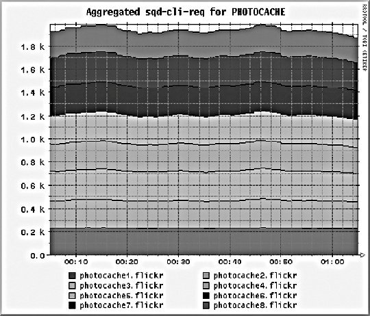 From this graph we can see that we're performing a total of around 2,000 Squid client requests per second, with an even spread on each of the eight nodes. If one band were thicker or thinner than another, we'd know that the particular node was being given an unfair shard of traffic. For some statistics, in addition to aggregating the counts from each node in a cluster, we want to compare several statistics on the same graph, as shown inFigure 10-11. Figure 10-11. Combining multiple statistics in a single graph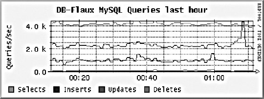 By looking at MySQL query rates side by side, we can see how many selects, inserts, updates, and deletes we're performing in relation to each other. We can see from the graph above that we perform roughly one insert for every two updates and four selects. Towards the end of our graph, we can see that updates briefly jumped higher than selects. We can then use this information for cache tuning, since we know how many reads and write we're trying to perform. We can also track this statistic against code changes to see what effect each change has on our read write ratio. We can also display useful static data on the graphs, to allow easy comparison with the dynamic statistics we gather, as shown in FFigure 10-12. Figure 10-12. Combining static and dynamic statistics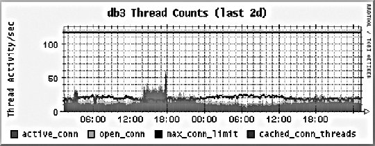 From this graph, we can see the number of open MySQL connections compared to the cache thread count. In addition, we can also see the maximum allowed connections (fixed at 118 in our example). By showing these together, we can easily see the active connections approaching the maximum limit and get a fast impression of how much thread capacity we have left. |