8.2. External Services and Black BoxesExternal services are the tricky component when removing bottlenecks. We can easily identify bottlenecks around external services, as we can profile how long we spend waiting for the services to respond. Before rushing to any conclusion about the speed of any services you're using, it's worth a sanity check to make sure they're really the problem. It's tempting to blame somebody else's service, but in the long run it's nearly always easier to address our own problems. Before looking at scaling the external service, we need to check that the way we're communicating with the service isn't causing the bottleneck. We can examine disk I/O and CPU as we read from and write to the service to check we're pushing out the request and pulling in the response fast enough. Once we're sure that the top of the network stack is all shiny, we can get down lower and check network latency and activity; perhaps our frames are colliding and never reaching the service until 200 ms after we make the request. Only once we're sure that the request is getting there hastily and the response is being received and parsed quickly do we start to blame the service. Solving the capacity question for external services depends very much on the nature of the service. Some services can be easily scaled out horizontally where multiple nodes are completely independent. Some services are designed for horizontal scaling, with infrastructure for node communication built in. Some services just won't scale. Unfortunately, if the latter is the case, then there's just not a lot you can do. 8.2.1. DatabasesIn a standard LAMP web application, the biggest bottleneck you'll find is database throughput, usually caused by disk I/O. This section comes last because while it's often the culprit and the first to receive attention, it's always a good idea to identify all of the contentions in your system before you start to optimize. When we talk about databases being a bottleneck, we're generally talking about the time between a query reaching the database server and its response being sent out. What we don't include is the time spent sending the query across the wire or receiving back the response data. This is the realm of network I/O contention and should always be investigated before starting with database optimization. Once we know that the problem lies within the database component, we can further narrow it down into a subset of the main query setthat is, the set of query classes that we run against the database. We'll first look at a couple of ways of finding the bottlenecks within our query set and then examine some methods for removing those bottlenecks. 8.2.2. Query Spot ChecksThe easiest way to start out database optimization is by building query spot checks into your database library. With spot checks, we enable a simple way to view the queries used by a single request, the SQL they contained, the server they were run on and the length of time they took. We assume that you're wrapping all of your application's database queries inside a single handler function that allows us to easily add hooks around all database operations. Inside our db_query( ) function, we add a couple of timing hooks and a call to display timing data:
function db_query($sql, $cluster){
       $query_start = get_microtime_ms( );
       $dbh = db_select_cluster($cluster);
       $result = mysql_query($sql, $dbh);
       $query_end = get_microtime_ms( );
       $query_time = $query_end - $query_start;
       $GLOBALS[debug][db_query_time] += $query_time;
       $GLOBALS[debug][db_query_count]++;
       db_debug("QUERY: $cluster - $sql ({$query_time}ms)");
}
function db_debug($message){
        if ($GLOBALS[config][debug_sql]){
                echo '<div class="debug">'.HtmlSpecialChars($message).'</div>';
        }
}
function get_microtime_ms( ){
        list($usec, $sec) = explode(" ", microtime( ));
        return round(1000 * ((float)$usec + (float)$sec));
}
Each time we perform a query, we can optionally output the SQL and timing data, aggregating the time and query count into global variables for outputting at the end of the request. You can then add a simple hook in your development and staging environments to activate debug output mode by appending a get parameter to the query string. The code might look something like this: $GLOBALS[config][debug_sql] = ($_GET[debug_sql] && $GLOBALS[config][is_dev_env]) ? 1 : 0; By then adding ?debug_sql=1 to the end of any request URL, we get a dump of all the queries executed, their timings, the total query count, and the total query time. You can add similar hooks to time the fetching of result sets to see how long you're spending communicating with the database in total. For large applications, finding the code that's executing a particular piece of SQL can be difficult. When we see a query running in the process list on the database server it's even harderwe don't know the request that triggered the query, so tracking it down can mean grepping through the source, which can be difficult if the query was constructed in multiple parts. With PHP 4.3 we have a fairly elegant solution. MySQL lets us add comments to our queries using the /* foo */ syntax. These comments show up inside the process list when a query is running. PHP lets us get a stack trace at any time, so we can see our execution path and figure out how we got to where we are. By combining these, we can add a simplified call chain to each SQL query, showing us clearly where the request came from. The code is fairly simple:
function db_query($sql, $cluster){
        $sql = "/* ".db_stack_trace( )." */ $sql";
        ...
}
function db_stack_trace( ){
        $stack = array( );
        $trace = debug_backtrace( );
        # we first remove any db_* functions, since those are
        # always at the end of the call chain
        while (strstr($trace[0]['function'], 'db_')){
                array_shift($trace);
        }
        # next we push each function onto the stack
        foreach($trace as $t){
                $stack[] = $t['function'].'( )';
        }
        # and finally we add the script name
        $stack[] = $_SERVER[PHP_SELF];
        $stack = array_reverse($stack)

        # we replace *'s just incase we might escape
        # out of the SQL comment
        return str_replace('*', '', implode(' > ', $stack));
}
We assemble a list of the call chain, removing the calls inside the database library itself (because every query would have these, they're just extra noise) and prepend it to the SQL before passing it to the database. Now any time we see the query, either in query spot checks or the database-process list, we can clearly see the code that executed it. Query spot checks are a really great tool for figuring out why a single page is acting slow or auditing a whole set of pages for query performance. The downside is that performing spot checks is not a good general query optimization technique. You need to know where to look for the slow queries and sometimes outputting debug information from them isn't easy. For processes that require a HTTP POST, adding a query parameter can be tricky, although PHP's output_add_rewrite_var( ) function can be a useful way to add debugging information to all forms at the cost of a performance drop. For processes that get run via cron, there's no concept of adding query parameters, other than via command-line switches. This can quickly get ugly. With the stack traces prepended to each query, we can watch the process list to spot queries that are taking too long. When we see a query that's been running for a couple of seconds, we can check the stack trace, dig down into the relevant code, and work on that query. This is a good quick technique for finding slow-running queries as they happen, but doesn't help us find the queries that have been running for 100 ms instead of 5 ms. For problems on that scale, we're going to need to create some tools. 8.2.3. Query ProfilingTo understand what queries we're executing and how long they're taking as a whole, we need to find out exactly what queries are running. While grepping through the source code and extracting SQL might sound like an interesting proposition at first, it misses some important data, such as how often we're calling each of the queries, relatively. Luckily for us, MySQL has an option to create a log of all the queries it runs. If we turn on this log for a while (which unfortunately requires a restart), then we can get a snapshot of the queries produced by real production traffic. The query log looks something like this:
/usr/local/bin/mysqld, Version: 4.0.24-log, started with:
Tcp port: 3306  Unix socket: /var/lib/mysql/mysql.sock
Time                 Id Command    Argument
050607 15:22:11        1 Connect     www-r@localhost on flickr
          1 Query       SELECT * FROM Users WHERE id=12
          1 Query       SELECT name, age FROM Users WHERE group=7
          1 Query       USE flickr_data
          1 Query       SELECT (prefs & 43932) != 0 FROM UserPrefs WHERE name=
'this user'
          1 Query       UPDATE UserPrefs SET prefs=28402 WHERE id=19
050607 15:22:12
          1 Quit
We want to extract only the SELECT queries, since we don't want to change our production data and we need queries to execute correctly. If we were really serious about profiling the write queries, then we could take a snapshot of the database before we started writing the query log so that we have a consistent set of data to run the profiling over. If you have a large dataset, snapshotting and rolling back data is a big task, worth avoiding. Of course, it's always a good idea to check through your snapshot restore sequence before you need to use it on your production setup. Once we've extracted a list of the select queries (a simple awk sequence should extract what we need), we can run them through a short benchmarking script. The script connects to the database (don't use a production server for this), disables the query cache (by performing SET GLOBAL query_cache_type = 0;), and performs the query. We time how long the query took by taking timestamps on either side of the database call. We then repeat the execution test a few times for the query to get a good average time. Once we've run the first query a few times, we output the SQL and average time taken, and move on to the next query. When we've completed all the queries, we should have an output line for every statement in the source log. At this point, it can be helpful to identify the query classes. By query class, we mean the contents of the query, minus any constant values. The following three queries would all be considered to be of the same query class: SELECT * FROM Frobs WHERE a=1; SELECT * FROM Frobs WHERE a=123; SELECT * FROM Frobs WHERE a='hello world'; We can then import the aggregated query class results into a spreadsheet and calculate a few key statistics for each query class: the query, the average time spent executing it, and the number of times it was executed. Query classes that took the largest amount of aggregated time will probably benefit from your attention first. The greater the number of times a query is executed, the greater total saving you'll achieve by speeding the query up by a certain amount. With a query log snapshot and expected results handy, we can build a regression test suite for database schema changes. Whenever we change a table's schema, we can rerun the test suite to see if there's an overall performance increase or decrease and look at elements that got slower as a result of the change. The suite then stops you from regressing previous query speed improvements when working on new indexes. 8.2.4. Query and Index OptimizationWe've used spot checks and query profiling to find the queries that are slowing us down and have now hopefully figured out which queries can be improved to increase overall system speed. But what should we be doing with these queries to make them faster? The first step in speeding up database performance is to check that we're making good use of the database indices. Designing the correct indices for your tables is absolutely essential. The difference between an indexed query and a nonindexed query on a large table can be less than a millisecond compared to several minutes. Because designing indexes is often so important to the core functioning of your application, it's an area for which you might consider hiring an experienced contractor to help you optimize your queries. In this case, it's important that you find somebody who's experienced in using your particular version of your particular database software. Oracle uses indexes in a very different way than MySQL, so an Oracle DBA isn't going to be a lot of immediate use. Although the field of query optimization even just within MySQL is big and complex, we'll cover the basics here to get you started and over the first of the major hurdles. For more information about query optimization, the query optimizer, index types, and index behavior you should check out High Performance MySQL (O'Reilly). MySQL allows you to use one index per table per query. If you're joining multiple tables, you can use one index from each. If you're joining the same table multiple times in the same query, then you can use one index for each join (they don't have to be the same index). MySQL has three main index typesPRIMARY KEY, UNIQUE, and INDEX. A table may only have one PRIMARY KEY index. All fields in the index must be nonnull, and all rows must have unique values in the index. The primary index always comes first in the index list. For InnoDB tables (which we'll look at in Chapter 9), the rows are stored on disk, ordered of the primary index (this is not the case for MyISAM tables). After the primary index come UNIQUE indexes. All rows must have a unique value, unless a column value is null. Finally come the regular INDEX indexes. These can contain multiple rows with the same value. We can find out what indexes MySQL is choosing to use by using the EXPLAIN statement. We use EXPLAIN in front of SELECT statements, with otherwise the same syntax. EXPLAIN then tells us a little about how the query optimizer has analyzed the query and what running the query will entail. The following sample query outputs a table of explanation: mysql> EXPLAIN SELECT * FROM Photos WHERE server=3 ORDER BY date_taken ASC; +--------+------+---------------+------+---------+------+----------+----------------+ | table | type | possible_keys | key | key_len | ref | rows | Extra | +--------+------+---------------+------+---------+------+----------+----------------+ | Photos | ALL | NULL | NULL | NULL | NULL | 21454292 | Using where; | | Using filesort | +--------+------+---------------+------+---------+------+----------+----------------+ We get one row for each table in the query (just one in this example). The first column gives us the table name, or alias if we used one. The second column shows the join type, which tells you how MySQL will find the results rows. There are several possible values, mostly relating to different multitable joins, but there are four important values for single table queries. const says that there is at most one matching rows, and it can be read directly from the index. This can only happen when the query references all of the fields in a PRIMARY or UNIQUE index with constant values. const lookups are by far the fastest, except the special case of system, where a table only has one row. Not as good as const, but still very fast, are range lookups, which will return a range of results read directly from an index. The key_len field then contains the length of the portion of the key that will be used for the lookup. When MySQL can still use an index but has to scan the index tree, the join type is given as index. While not the worst situation, this isn't super fast like a range or const. At the very bottom of our list comes the ALL type, given in capital letters to reflect how scary it is. The ALL type designates that MySQL will have to perform a full table scan, examining the table data rather than the indexes. Our example query above is not so great. The possible_keys column lists the indexes that MySQL could have used for the query, while the key column shows the index it actually chose, assuming it chose one at all. If MySQL seems to be picking the wrong index, then you can set it straight by using the USE INDEX( ) and FORCE INDEX( ) syntaxes. The key_len column shows how many bytes of the index will be used. The ref column tells us which fields are being used as constant references (if any), while the rows column tells us how many rows MySQL will need to examine to find our results set. Our example query could certainly use some optimization: as it is now, MySQL is going to have to perform a table scan on 20 million rows. The final column gives us some extra pieces of information, some of which are very useful. In our example we get Using where, which tells us we're using a WHERE clause to restrict results. We expect to see this most of the time, but if it's missing we know that the query optimizer has optimized away our WHERE clause (or we never had one). The value Using filesort means that the rows MySQL finds won't be in the order we asked for them, so a second pass will be needed to order them correctly. This is generally a bad thing and can be overcome with careful indexing, which we'll touch on in a moment. If you ask for complex ordering or grouping, you might get the extra value of Using temporary, which means MySQL needed to create a temporary table for manipulating the result set. This is generally bad. On the good side, seeing Using index means that the query can be completed entirely from index without MySQL ever having to check row data; you should be aiming to have this status for all tables that aren't trivially small. Depending on the fields that result in a SELECT statement, MySQL can in some cases return results without looking at the table rows; this is often referred to as index covering. If the fields you request are all within the index and are being used in the WHERE clause of the query, MySQL will return results straight from the index, significantly speeding up the query and reducing disk I/O. Let's add an index for our previous example query to use: mysql> ALTER TABLE Photos ADD INDEX my_index (server, date_taken); Query OK, 21454292 rows affected (9726 sec) Records: 21454292 Duplicates: 0 Warnings: 0 mysql> EXPLAIN SELECT * FROM Photos WHERE server=3 ORDER BY date_taken ASC; +--------+------+---------------+----------+---------+-------+---------+------------+ | table | type | possible_keys | key | key_len | ref | rows | Extra | +--------+------+---------------+----------+---------+-------+---------+------------+ | Photos | ref | my_index | my_index | 2 | const | 1907294 | Using where| +--------+------+---------------+----------+---------+-------+---------+------------+ We created an index and now we use a key, perform a ref join, and don't need to perform a file sort. So let's look at how the index is working. MySQL uses the fields in indexes from left to right. A query can use part of an index, but only the leftmost part. An index with the fields A, B, and C can be used to perform lookups on field A, fields A and B, or fields A, B, and C, but not fields B and C alone. We can create a sample table to test our understanding of index handling using the following SQL statement: CREATE TABLE test_table ( a tinyint(3) unsigned NOT NULL, b tinyint(3) unsigned NOT NULL, c tinyint(3) unsigned NOT NULL, KEY a (a,b,c) ); The index is best utilized when the non-rightmost fields are constant references. Using our example index we can ask for a range of values from field B as long as we have a constant reference for column A: Good: SELECT * FROM test_table WHERE a=100 AND b>50; Bad: SELECT * FROM test_table WHERE a<200 AND b>50; The results are ordered in the index by each field, left to right. We can make use of this ordering in our queries to avoid a file sort. All leftmost constant referenced fields in the index are already correctly sorted, as is the field following the last constantly referenced field (if any). The following examples, using our example table, show the situations in which the index can be used for the sorting of results: Good: SELECT * FROM test_table ORDER BY a; Bad: SELECT * FROM test_table ORDER BY b; Bad: SELECT * FROM test_table ORDER BY c; Good: SELECT * FROM test_table WHERE a=100 ORDER BY a; Good: SELECT * FROM test_table WHERE a=100 ORDER BY b; Bad: SELECT * FROM test_table WHERE a=100 ORDER BY c; Good: SELECT * FROM test_table WHERE a>100 ORDER BY a; Bad: SELECT * FROM test_table WHERE a>100 ORDER BY b; Bad: SELECT * FROM test_table WHERE a>100 ORDER BY c; Good: SELECT * FROM test_table WHERE a=100 AND b=100 ORDER BY a; Good: SELECT * FROM test_table WHERE a=100 AND b=100 ORDER BY b; Good: SELECT * FROM test_table WHERE a=100 AND b=100 ORDER BY c; Good: SELECT * FROM test_table WHERE a=100 AND b>100 ORDER BY a; Good: SELECT * FROM test_table WHERE a=100 AND b>100 ORDER BY b; Bad: SELECT * FROM test_table WHERE a=100 AND b>100 ORDER BY c; By creating test tables, filling them with random data, and trying different query patterns, you can use EXPLAIN to infer a lot about how MySQL optimizes indexed queries. There's nothing quite like trial and error for figuring out what index will work best, and creating a test copy of your production database for index testing is highly recommended. Unlike other commercial databases, MySQL doesn't pay a lot of attention to the distribution of data throughout an index when selecting the right index for the job, so the randomness of the sample data shouldn't affect you too much, unless your data distribution is wildly skewed. However, MySQL will skip using indexes altogether if the table has too few rows, so it's always a good idea to stick a couple of thousand rows in your test tables and make sure your result sets are reasonably large. Just bear in mind these simple rules when working with MySQL indexes:
8.2.5. CachingCertain kinds of data are ripe for caching: they get set very infrequently but fetched very often. Account data is often a good example of thisyou might want to load account data for every page that you display, but you might only edit account data during 1 in every 100 requests. If we can move this traffic away from the database, then we can free up CPU and I/O bandwidth for other processing that must be run via the database. We can implement a simple cache as yet another layer in our software architecture model, shown in Figure 8-7. Figure 8-7. Adding caching to our software architecture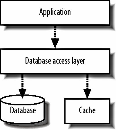 When we go to fetch an object, we first check in the cache. If the object exists, we read it from the cache and return it to the requesting process. If it doesn't exist in cache, we read the object from the database, store it in the cache, and return it to the requestor. When we go to change an object in the database, either for an update or a delete, we need to invalidate the cache. We can either just drop the object from cache or update it in place by fetching the currently cached version, updating it in the same way the SQL will update the version in the database, and restoring it in the cache. The latter technique also means that objects become cached after a change, which is probably what you wanted, since an object being modified will probably need to be accessed shortly afterward. memcached (memory cache daemon, pronounced mem-cache-dee; http://www.danga.com/memcached/) is a generic open source memory-caching system designed to be used in web applications to remove load from database servers. memcached supports up to 2 GB of cache per instance, but allows you to run multiple instances per machine and spread instances across multiple machines. Native APIs are available for PHP, Perl, and a whole host of other common languages. It's extremely important that we correctly invalidate the data in the cache when we change the primary version in the database. Stale data in the cache will give us some very strange errors, such as edits we've performed not appearing, new content not appearing, and old, deleted content not disappearing. For the same reason, it's very important we don't populate a cache with stale data, since it won't have a chance of being corrected unless we edit the object again. If you're using MySQL in a replicated setup, which we'll discuss in Chapter 9, then you'll always want to populate your cache from the master. Depending on the nature of the data you're caching, you may not need to invalidate the cached copy every time you update the database. In the case of variables that aren't visible to application users and aren't used to determine interaction logic, such as administrative counters, we don't care if the cached copy is completely up-to-date, as long as the underlying database is accurate. In this case we can skip the cache invalidation, which increases the cache lifetime of our objects and so reduces the query rate hitting the database. If the objects you're caching have multiple keys by which they're accessed, you might want to store the objects in a cache tied to more than one key. For instance, a photo belonging to user 94 might be cached as record number 9372, but also as the second photo belonging to the user. We can then create two keys for the object to be cached underphoto_9372 and user_94_photo_2. Most simple cache systems deal in key/value pairs, with a single key accessing a single value. If we were to store the object under each key, we'd be using twice as much the space as we would storing it under one key, and any update operations would require twice as much work. Instead, we can designate one of the keys to be the primary, under which we store the actual object. In our example, the key photo_9372 would have the serialized photo object as the value. The other keys can then have values pointing to the primary key. Following the example, we'd store the key user_94_photo_2 with a value of photo_9372. This increases the cost of lookups for nonprimary keys slightly, but increases the number of objects we can store in the cache and reduces the number of cache updates. Since reads are typically very cheap, while writes and space aren't, this can give a significant performance increase compared to storing the object twice. Remember, the more space in our cache, the more objects we can cache, the fewer objects fall out of cache, and the fewer requests go through to the database. Read caching in this way can be a big boost for database-driven applications, but has a couple of drawbacks. First, we're only caching reads, while all writes need to be written to the database synchronously and the cache either purged or updated. Second, our cache-purging and updating logic gets tied into our application and adds complexity. The outcome of this complexity often manifests itself as code that updates the database but fails to correctly update the cache, resulting in stale objects. Carrying on with our theme of layers, we can instead implement a cache as an entire layer that sits between the application and the database, as shown in Figure 8-8. Figure 8-8. Treating caches as a layer of their own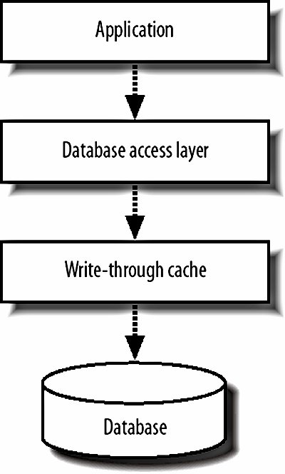 We call this a write-through cache; all writes come through it, which allows the cache to buffer writes together and commit them in batches, increasing the speed by decreasing concurrency. Because the cache layer only contains code for reading and writing data and no higher application logic, it can be built as a fairly general purpose application. As such, it's a much easier task to ensure that a fresh copy of the data is always served out. The cache knows about every update operation and the underlying database cannot be modified without the cache knowing about it. The downside to such a system is raw complexity. Any write-through cache will have to support the same feature set our application is expecting from the database below it, such as transactions, MVVC, failover, and recovery. Failover and recovery tend to be the big showstoppersa cache must be able to suffer an outage (machine crash, network failure, power outage, etc.) without losing data which had been "written" by the application, at least to the extent that the remaining data is in a consistent state. This usually entails journaling, check summing, and all that good stuff that somebody else already took the time to bake into the database software. Getting more performance from a caching layer is fairly straightforwardwe just need to add more space in the cache by adding more memory to the machine. At some point, we'll either run out of memory (especially on 32-bit boxes) or we'll saturate the machine's network connection. To grow the cache past this point, we simply add more boxes to the cache pool and use some algorithm to choose which particular box should handle each key. A layer 7 load balancer (we'll see more of those in Chapter 9) can do that job for us if we're worried about a machine failing; otherwise, we can compute a simple hash based on the key name, divide it modulo the number of machines in the cache pool, and use the resulting numbered server. 8.2.6. DenormalizationThe final line of pure database performance optimization, before we start to talk about scaling, is data denormalization. The idea behind denormalization is very simplecertain kinds of queries are expensive, so we can optimize those away by storing data in nonnormal form with some pieces of data occurring in multiple places. Database indexes can be regarded as a form of denormalization: data is stored in an alternative format alongside the main row data, allowing us to quickly perform certain operations. The database takes care of keeping these indexes in sync with the data transparently. We'll use a very simple example to demonstrate what we mean. We have a forum application that allows users to create discussion topics and gather replies. We want to create a page that shows the latest replies to topics we started, so we do a simple join: SELECT r.* FROM Replies AS r, Topics AS t WHERE t.user_id=100 AND r.topic_id=t.id ORDER BY r.timestamp DESC This is all well and good and will give us the correct results. As time goes by and our tables get bigger and bigger, performance starts to degrade (it's worth noting that MySQL has lousy join performance for huge tables, even when correctly indexed). Opening two indexes for this task is overkillwith a little denormalization we can perform a single simple select. If we add the ID of the topic creator to each reply record, then we can select straight from the reply table: SELECT * FROM Replies WHERE topic_user_id=100 ORDER BY timestamp DESC The index we need is very straightforward; a two-column index on topic_user_id and timestamp. Cardinality of the index will be good since we'll only ever be selecting rows from topics we started, with the index skipping straight to them. There are downsides to this approach, though, as any CS major will tell you. The relational database is designed to keep our data relational and consistent. If the correct value isn't set for the topic_user_id column, then our data will be out of sync and inconsistent. We can use transactions to ensure that they're changed together, but this doesn't stop us from creating reply rows with incorrect values. The real problem stems from the fact that we're now relying on our specialized code to provide and ensure the consistency and our code is fallible. At a certain scale, denormalization becomes more and more essential. A rigorous approach to separation of interaction and business logic can help to ensure that denormalization takes place consistently, but problems can always slip through. If you plan to have denormalized data in your application, building tools to verify and correct the denormalized data will save you a lot of time. In our above example, if we suspected that the data was out of sync, we could run a checking tool that verified each row to check for inconsistencies. If one turns up, we can find the problem in our code and redeploy. Once the fixed code is live, we can then run a repair tool to correct the out of sync data. For our example, the check and repair steps can each be a single query, but complex denormalized data may need much more involved scripts. What we haven't mentioned here is the use of stored procedures and triggers to automatically keep data denormalized for us. In our example situation above, we would insert a row of data into the replies table and an insert trigger would automatically update the topic_user_id value. Another trigger would watch the user_id value in the topics table, ready to update the replies table if the value changes. This can be quite a big help, but still suffers from the same problem as keeping denormalization node in your business logicit's not infallible. You can easily miss a needed trigger, set the trigger up incorrectly, or make a mistake in the stored procedure. A further argument against using stored procedures is that it moves a partial block of logic out of the business logic layer. Because the business logic layer will be selecting from the denormalized field, it's out of place that another layer creates the values in that field. This over-separation can make systems more complicated, which then leads to further errors. Besides, if we're using MySQL 4, then we don't have the luxury of either stored procedures or triggers. MySQL 5 will have both, but is not currently production-ready and might not be for some time. PostgreSQL and Oracle have both, with Oracle offering its crazy PL/SQL language. But there's nothing we can do with triggers and stored procedures that we can't do in code (although it'll typically be harder and more error prone), so it's not time to give up on MySQL just yet. |